Execution Plan Cache Analysis

Execution Plan Generation

SQL Server uses a cost-based optimization technique to determine the processing strategy of a query. The optimizer considers both the metadata of the database objects, such as unique constraints or index size, and the current distribution statistics of the columns referred to in the query when deciding which index and join strategies should be used.

The following techniques are performed in order :

• Parsing
• Binding
• Query optimization
• Execution plan generation, caching, and hash plan generation
• Query execution

In order to arrive at an optimal plan, the query optimizer uses transformation rules and heuristics. The optimizer uses heuristics to reduce the amount of available optimization options. The plans are stored in memory is a component called the Memo. The optimizer adopts different techniques, namely, the following:

• Simplification
• Trivial plan match
• Multiple optimization phases
• Parallel plan optimization

View Query Tree

We can use some undocumented query hints and view the query that sql server optimizaer generates as follows :

SELECT Count(*)
FROM Person.Person
OPTION (RECOMPILE,  QUERYTRACEON 8606, QUERYTRACEON 3604, QUERYTRACEON 8612, QUERYTRACEON 2372);
-- QUERYTRACEON 3604 Output to console
-- QUERYTRACEON 8606 Logical operators trees
-- QUERYTRACEON 8612   -- Add aditional cardinality info
-- QUERYTRACEON 2372,  -- Optimization stage memory info

Costing the Plan

The query optimizer estimates the cost of each operator in the query tree and selects the least expensive one. SQL Server estimates the number of rows returned, cardinality estimate, by looking at the statistics available. It also considers the resources such as I/O, CPU and memory used by each operator.

Components of the Execution Plan

The execution plan generated by the optimizer contains two components.

• Query plan - This represents the commands that specify all the physical operations required to execute a query.
• Execution context - This maintains the variable parts of a query within the context of a given user.

Aging of the Execution Plan

The procedure cache is part of SQL Server’s buffer cache, which also holds data pages. As new execution plans are added to the procedure cache, the size of the procedure cache keeps growing, affecting the retention of useful data pages in memory. To avoid this, SQL Server dynamically controls the retention of the execution plans in the procedure cache, retaining the frequently used execution plans and discarding plans that are not used for a certain period of time.

When an execution plan is generated, the age field is populated with the cost of generating the plan. A complex query requiring extensive optimization will have an age field value higher than that for a simpler query.

The cheaper the execution plan was to generate, the sooner its cost will be reduced to 0. Once an execution plan’s cost reaches 0, the plan becomes a candidate for removal from memory.

Analyzing the Execution Plan Cache

You can obtain a lot of information about the execution plans in the procedure cache by accessing various dynamic management objects. The initial DMO for working with execution plans is sys.dm_exec_cached_plans.

SELECT  *
FROM    sys.dm_exec_cached_plans;

Execution Plan Reuse

When a query is submitted, SQL Server checks the procedure cache for a matching execution plan. If one is not found, then SQL Server performs the query compilation and optimization to generate a new execution plan. However, if the plan exists in the procedure cache, it is reused with the private execution context. This saves the CPU cycles that otherwise would have been spent on the plan generation.

Query Plan Hash and Query Hash

With SQL Server 2008, new functionality around execution plans and the cache was introduced called the query plan hash and the query hash. These are binary objects using an algorithm against the query or the query plan to generate the binary hash value.

To see the hash values in action, create two queries.

SELECT  *
FROM    Production.Product AS p
JOIN    Production.ProductSubcategory AS ps
        ON p.ProductSubcategoryID = ps.ProductSubcategoryID
JOIN    Production.ProductCategory AS pc
        ON ps.ProductCategoryID = pc.ProductCategoryID
WHERE   pc.[Name] = 'Bikes'
        AND ps.[Name] = 'Touring Bikes';

SELECT  *
FROM    Production.Product AS p
JOIN    Production.ProductSubcategory AS ps
        ON p.ProductSubcategoryID = ps.ProductSubcategoryID
JOIN    Production.ProductCategory AS pc
        ON ps.ProductCategoryID = pc.ProductCategoryID
where   pc.[Name] = 'Bikes'
        and ps.[Name] = 'Road Bikes';

After you execute each of these queries, you can see the results of these format changes from sys.dm_exec_query_stats :

SELECT  deqs.execution_count,
        deqs.query_hash,
        deqs.query_plan_hash,
        dest.text
FROM    sys.dm_exec_query_stats AS deqs
CROSS APPLY sys.dm_exec_sql_text(deqs.plan_handle) dest
WHERE   dest.text LIKE 'SELECT  *
FROM    Production.Product AS p%';

Query Plan Caching

The execution plan of a query generated by the optimizer is saved in a special part of SQL Server’s memory pool called the plan cache or procedure cache. Saving the plan in a cache allows SQL Server to avoid running through the whole query optimization process again when the same query is resubmitted. SQL Server supports different techniques such as plan cache aging and plan cache types to increase the reusability of the cached plans. It also stores two binary values called the query hash and the query plan hash.

When performing query tuning, you will need to clear the plan cache. You can use the DBCC command as follows :

DBCC FREEPROCCACHE

View Cached Query Plan

We can view the cached query plans using the DMV sys.dm_exec_cached_plans as follows :

SELECT usecounts, cacheobjtype, plan_handle
FROM sys.dm_exec_cached_plans
WHERE cacheobjtype = 'Compiled Plan'

View Graphical Execution Plan from Cache

We can use the stored binary plan handle to retrieve the XML and graphical query plans using the DMF sys.dm_exec_query_plan and passing the plan handle as follows :

SELECT query_plan 
FROM sys.dm_exec_query_plan(<query plan handle here>)

View Memory Used by Cached Plans

We can use the sys.dm_os_memory_cache_entries to see the memory used by cached query plans for both Adhoc queries, stored procedures and bound tree with the following :

SELECT name, in_use_count, original_cost, pages_kb
FROM sys.dm_os_memory_cache_entries
WHERE type in ('CACHESTORE_OBJCP', 'CACHESTORE_SQLCP', 'CACHESTORE_PHDR')

Reading Query Plans

SQL Server supports displaying the query plans as :

• Graphical
• Text
• XML

Display Graphical Query Plan

Using SQL Server Management Studio we can display two types of the execution plan :

• Estimated Execution Plan
• Actual Execution Plan

Running the following query on my machine :

USE AdventureWorks2012
GO
SELECT DISTINCT(City)
FROM Person.Address

i get the following execution plan.

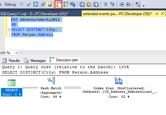
Characterstics

• Each node represents an operation implemented by an iterator, also called an operator. The logical operation is displayed in brackets. If both logical and physical are the same no brackets are displayed.
• Each node is related to its parent, and data flow is represented with arrows
• Data flows from left to right
• The arrow width represents the relative number of rows returned
• You can hover on the operator for more properties

To perform their job, physical operators implement at least the following three methods:

• Open() - Causes an operator to be initialized, and may include setting up any required data structures
• GetRow() - Requests a row from the operator
• Close() - Performs some cleanup operations and shuts down the operator once it has performed its role

Display Text Plan

The text plans will be deprecated in future, instead you should use the XML and graphical execution plan. The two options allow you to display estimated execution plans as text. We can also display query plan as text using the SET option SHOWPLAN_TEXT and setting to ON and OFF as follows:

USE AdventureWorks2012
GO
SET SHOWPLAN_TEXT ON
GO
SELECT DISTINCT(City) 
FROM Person.Address
GO
SET SHOWPLAN_TEXT OFF

and we will get the follwing output :

StmtText
----------------------------------------------
SELECT DISTINCT(City) 
FROM Person.Address

(1 row(s) affected)

StmtText
----------------------------------------------------------------------------------------------------------------------------------------------------------------------------------------------
  |--Hash Match(Aggregate, HASH:([AdventureWorks2012].[Person].[Address].[City]), RESIDUAL:([AdventureWorks2012].[Person].[Address].[City] = [AdventureWorks2012].[Person].[Address].[City]))
       |--Index Scan(OBJECT:([AdventureWorks2012].[Person].[Address].[IX_Address_AddressLine1_AddressLine2_City_StateProvinceID_PostalCode]))

(2 row(s) affected)

To display additional information, you can use the SHOWPLAN_ALL SET option as follows :

USE AdventureWorks2012
GO
SET SHOWPLAN_ALL ON
GO
SELECT DISTINCT(City) 
FROM Person.Address
GO
SET SHOWPLAN_ALL OFF

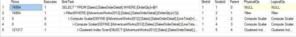
The STATISTICS PROFILE SET options actually runs the query and displays the text plan with more detailed results as follows :

Use AdventureWorks2012
GO
SET STATISTICS PROFILE ON
GO
SELECT DISTINCT(City)
FROM Person.Address
GO
SET STATISTICS PROFILE OFF

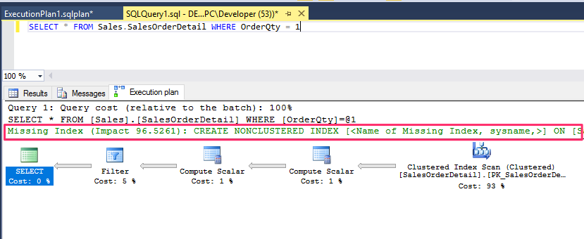
Missing Indexes from Graphical Execution

The graphical query execution plan can show when a query can benefit from missing indexes.

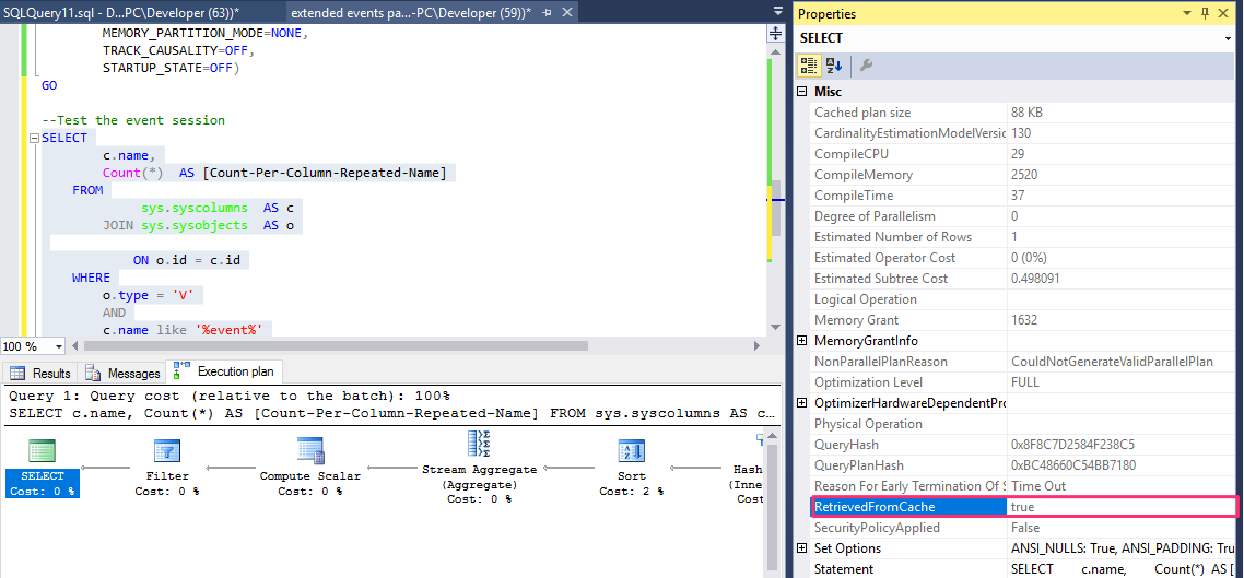
Additional Plan Properties

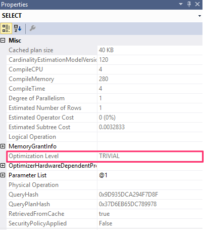
The query plan properties also display the reason for an early termination in the Optimization Level property, e.g when we run the following query :

SELECT * FROM Sales.SalesOrderHeader
WHERE SalesOrderID = 43666

you will notice that the level is displayed as a trivial as follows :

but we can use a query hint to disable the trivial plan instead as follows :

SELECT * FROM Sales.SalesOrderHeader
WHERE SalesOrderID = 43666
OPTION (QUERYTRACEON 8757)

The CardinalityEstimationModelVersion attribute refers to the version of the cardinality estimation model used by the query optimizer. SQL Server 2014 introduces a new cardinality estimator, but you still have the choice of using the old one by changing the database compatibility level or using trace flags 2312 and 9481.

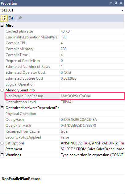
The NonParallelPlanReason optimal gives a reason why a parallel plan was not chosen. E.g if we use the option hint to use only one processor by setting the MAXDOP to 1 as follows :

SELECT * FROM Sales.SalesOrderHeader
WHERE SalesOrderID = 43666
OPTION (MAXDOP 1)

Warnings on Execution Plans

The query plan also shows warnings and these should be carefully reviewed. The following warnings are displayed :

• ColumnsWithNoStatistics
• NoJoinPredicate
• SpillToTempDb
• TypeConversion
• Wait
• PlanAffectingConvert
• SpatialGuess
• UnmatchedIndexes
• FullUpdateForOnlineIndexBuild

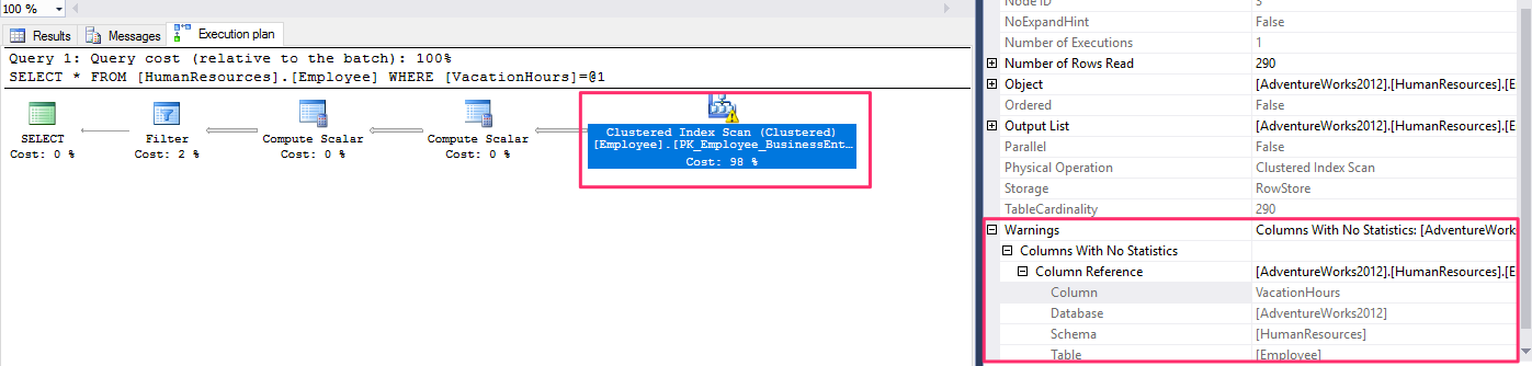
ColumnsWithNoStatistics Warning

They were no statistics available to the query optimizer for the column.

Run the following statement to drop the existing statistics for the VacationHours column, if available:

DROP STATISTICS HumanResources.Employee._WA_Sys_0000000C_49C3F6B7

We can view the statistics on the table with the following query :

SELECT s.name, c.name, auto_created 
FROM sys.stats s
JOIN sys.columns c
ON s.object_id = c.object_id and s.stats_id = c.column_id
WHERE s.object_id = object_id('HumanResources.Employee')

Next, temporarily disable automatic creation of statistics at the database level:

ALTER DATABASE AdventureWorks2012
SET AUTO_CREATE_STATISTICS OFF

Then run this query:

SELECT * FROM HumanResources.Employee
WHERE VacationHours = 48

and you will get a query plan as follows :

Enable the auto creating of statistics with the following :

ALTER DATABASE AdventureWorks2012 SET AUTO_CREATE_STATISTICS ON

and re-run the query. You will notice the query plan no longer have warnings as the statistics have been auto created.

NoJoinPredicate Warning

A possible problem while using the old-style ANSI SQL-89 join syntax is accidentally missing the join predicate and getting a NoJoinPredicate warning. Let’s suppose you intend to run the following query but forgot to include the WHERE clause:

SELECT * FROM Sales.SalesOrderHeader soh, Sales.SalesOrderDetail sod WHERE soh.SalesOrderID = sod.SalesOrderID

The first indication of a problem could be that the query takes way too long to execute, even for small tables. Later, you will see that the query also returns a huge result set.

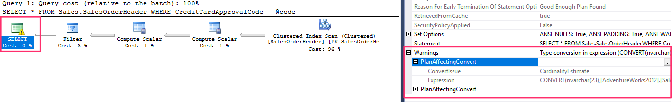
PlanAffectingConvert Warning

This warning shows that type conversions were performed that may impact the performance of the resulting execution plan. Run the following example, which declares a variable as nvarchar and then uses it in a query to compare against a varchar column, CreditCardApprovalCode:

DECLARE @code NVARCHAR(15)
SET @code = '95555Vi4081'
SELECT * 
FROM Sales.SalesOrderHeader
WHERE CreditCardApprovalCode = @code

SpillToTempDb Warning

This warning shows than an operation didn’t have enough memory and had to spill data to disk during execution, which can be a performance problem because of the extra I/O overhead. To simulate this problem, run the following example:

SELECT * FROM Sales.SalesOrderDetail ORDER BY UnitPrice

This is a very simple query, and depending on the memory available on your system, you may not get the warning in your test environment, so you may need to try with a larger table instead.

UnmatchedIndexes

Finally, the UnmatchedIndexes element can show that the query optimizer was not able to match a filtered index for a particular query (for example, when it is not able to see the value of a parameter). Suppose you create the following filtered index:

CREATE INDEX IX_Color ON Production.Product(Name, ProductNumber)
WHERE Color = ‘White’

and then run the query :

DECLARE @color nvarchar(15)
SET @color = 'White'
SELECT Name, ProductNumber FROM Production.Product
WHERE Color = @color

You will notice we get an unmatched index, however the following will use an index :

SELECT Name, ProductNumber FROM Production.Product
WHERE Color = 'White'

and remove the index :

DROP INDEX Production.Product.IX_Color

Getting Plans from the Plan Cache

Most of the times you will not run the queries manually but you will need to invest the queries that have already been ran. We can can retrieve the query plan in cache using the sys.sm_exec_cached_plans or from currently executing queries using sys.dm_exec_requests and from query statistics using sys.dm_exec_query_stats :

Retrive from current executing queries

-- A plan_handle is a hash value that represents a specific execution plan
SELECT * FROM sys.dm_exec_requests
CROSS APPLY
sys.dm_exec_query_plan(plan_handle)

From query stats

-- The sys.dm_exec_query_stats DMV contains one row per query statement within the cached plan
SELECT * FROM sys.dm_exec_query_stats
CROSS APPLY
sys.dm_exec_query_plan(plan_handle)

Retrieve top 10 queries by usage

-- You can run the following query to get this information
SELECT TOP 10 total_worker_time/execution_count AS avg_cpu_time,
plan_handle, query_plan
FROM sys.dm_exec_query_stats
CROSS APPLY sys.dm_exec_query_plan(plan_handle)
ORDER BY avg_cpu_time DESC

Removing Plans from the Plan Cache

• The DBCC FREEPROCCACHE statement can be used to remove all the entries from the plan cache.
• The DBCC FREESYSTEMCACHE statement can be used to remove all the elements from the plan cache or only the elements associated with a Resource Governor pool name.
• The DBCC FLUSHPROCINDB can be used to remove all the cached plans for a particular database.
• Not related, the DBCC DROPCLEANBUFFERS statement can be used to remove all the buffers from the buffer pool.

SET STATISTICS TIME / IO

You can use SET STATISTICS TIME to see the number of milliseconds required to parse, compile, and execute each statement. For example, run

SET STATISTICS TIME ON

and then run the following query:

SELECT DISTINCT(CustomerID)
FROM Sales.SalesOrderHeader

and turn it off :

SET STATISTICS TIME OFF

SET STATISTICS IO displays the amount of disk activity generated by a query. To enable it, run the following statement:

SET STATISTICS IO ON

Run this next statement to clean all the buffers from the buffer pool to make sure that no pages for this table are loaded in memory:

DBCC DROPCLEANBUFFERS

Then run the following query:

SELECT * FROM Sales.SalesOrderDetail WHERE ProductID = 870

It will show an output similar to the following:

Here are the definitions of these items, which all use 8K pages:

• Logical reads Number of pages read from the buffer pool.
• Physical reads Number of pages read from disk.
• Read-ahead reads Read-ahead is a performance optimization mechanism that anticipates the needed data pages and reads them from disk. It can read up to 64 contiguous pages from one data file.
• Lob logical reads Number of large object (LOB) pages read from the buffer pool.
• Lob physical reads Number of large object (LOB) pages read from disk.
• Lob read-ahead reads Number of large object (LOB) pages read from disk using the read-ahead mechanism, as explained earlier.

Now, if you run the same query again, you will no longer get physical and read-ahead reads.

Scan count is defined as the number of seeks or scans started after reaching the leaf level (that is, the bottom level of an index). The only case when scan count will return 0 is when you’re seeking for only one value on a unique index, like in the following example:

SELECT * FROM Sales.SalesOrderHeader WHERE SalesOrderID = 51119

If you try the following query, in which SalesOrderID is defined in a nonunique index and can return more than one record, you can see that scan count now returns 1:

SELECT * FROM Sales.SalesOrderDetail WHERE SalesOrderID = 51119

Finally, in the following example, scan count is 4 because SQL Server has to perform four seeks:

SELECT * FROM Sales.SalesOrderHeader WHERE SalesOrderID IN (51119, 43664, 63371, 75119)

Execution Plan Cache Recommendations

To ensure efficient use of the plan cache, follow these recommendations:

• Explicitly parameterize variable parts of a query.
• Use stored procedures to implement business functionality.
• Use sp_executesql to avoid stored procedure maintenance.
• Use the prepare/execute model to avoid resending a query string.
• Avoid ad hoc queries.
• Use sp_executesql over EXECUTE for dynamic queries.
• Parameterize variable parts of queries with care.
• Avoid modifying environment settings between connections.
• Avoid the implicit resolution of objects in queries.

Query Optimizer in-depth

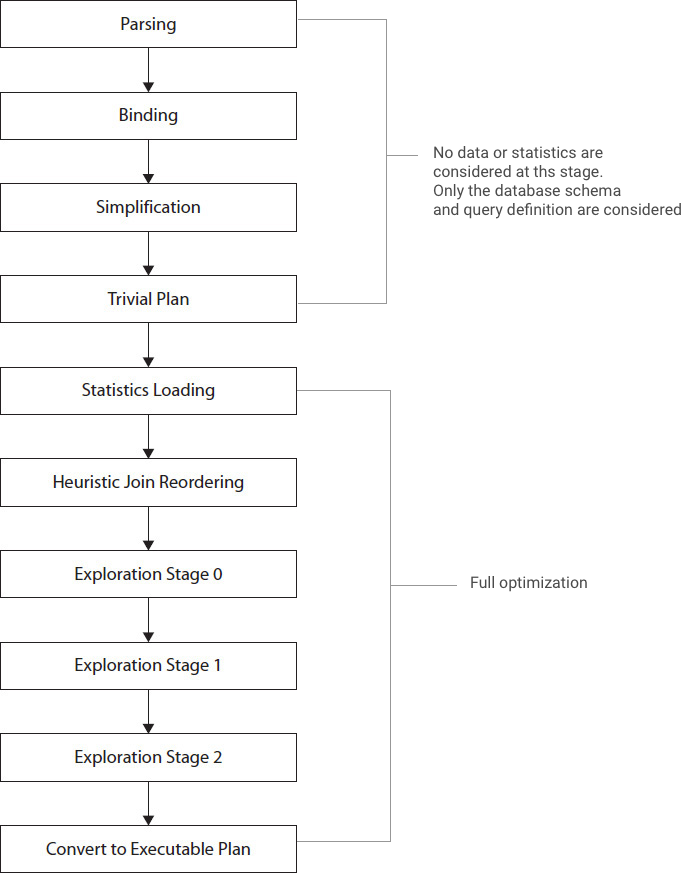
In this part we will now go in-depth and look at the query optimization process. Here is the major steps of the query optimization process.

DMVs for Query Optimization sys.dm_exec_query_optimizer_info

Returns detailed statistics about the operation of the SQL Server query optimizer. You can use this view when tuning a workload to identify query optimization problems or improvements. For example, you can use the total number of optimizations, the elapsed time value, and the final cost value to compare the query optimizations of the current workload and any changes observed during the tuning process. Some counters provide data that is relevant only for SQL Server internal diagnostic use.

Viewing statistics on optimizer execution

What are the current optimizer execution statistics for this instance of SQL Server?

SELECT * FROM sys.dm_exec_query_optimizer_info;

Name	Data type	Description
counter	nvarchar(4000)	Name of optimizer statistics event.
occurrence	bigint	Number of occurrences of optimization event for this counter.
value	float	Average property value per event occurrence.

Viewing the total number of optimizations

How many optimizations are performed?

SELECT occurrence AS Optimizations FROM sys.dm_exec_query_optimizer_info
WHERE counter = 'optimizations';

Average elapsed time per optimization

What is the average elapsed time per optimization?

SELECT ISNULL(value,0.0) AS ElapsedTimePerOptimization  
FROM sys.dm_exec_query_optimizer_info WHERE counter = 'elapsed time';  

Fraction of optimizations that involve subqueries

What fraction of optimized queries contained a subquery?

SELECT (SELECT CAST (occurrence AS float) 
FROM sys.dm_exec_query_optimizer_info WHERE counter = 'contains subquery') /  
(SELECT CAST (occurrence AS float) FROM sys.dm_exec_query_optimizer_info WHERE counter = 'optimizations')  
AS ContainsSubqueryFraction;

and as a percentage of the total optimizations :

SELECT (SELECT CAST (occurrence AS float) 
FROM sys.dm_exec_query_optimizer_info WHERE counter = 'contains subquery') /  
(SELECT CAST (occurrence AS float) FROM sys.dm_exec_query_optimizer_info WHERE counter = 'optimizations') * 100 
AS ContainsSubqueryFraction ;

View percentage of optimization on query with hints

This will be a good indicator on the flexibility of the application. The application should use hints sparingly.

-- for example, the next query displays the percentage of optimizations in the instance that include hints
SELECT (SELECT occurrence FROM sys.dm_exec_query_optimizer_info WHERE counter = 'hints' ) * 100.0 / 
(SELECT occurrence FROM sys.dm_exec_query_optimizer_info WHERE counter = 'optimizations' )

Check optimizations for a specific workload

We can use the DMV to check for the optimization applied to a specific workload but they are several issues. There is no easy way but we can get a snapshot of the before optimization and after optimization and subtract the value to have an idea of the optimizations applied.

Here is a query that can do that

-- optimize these queries now
-- so they do not skew the collected results
GO
SELECT *
INTO after_query_optimizer_info
FROM sys.dm_exec_query_optimizer_info
GO
SELECT *
INTO before_query_optimizer_info
FROM sys.dm_exec_query_optimizer_info
GO
DROP TABLE before_query_optimizer_info
DROP TABLE after_query_optimizer_info
GO
-- real execution starts
GO
SELECT *
INTO before_query_optimizer_info
FROM sys.dm_exec_query_optimizer_info
GO
-- insert your query here
SELECT *
FROM Person.Address
-- keep this to force a new optimization
OPTION (RECOMPILE)
GO
SELECT *
INTO after_query_optimizer_info
FROM sys.dm_exec_query_optimizer_info
GO
SELECT a.counter,
(a.occurrence - b.occurrence) AS occurrence,
(a.occurrence * a.value - b.occurrence *
b.value) AS value
FROM before_query_optimizer_info b
JOIN after_query_optimizer_info a
ON b.counter = a.counter
WHERE b.occurrence <> a.occurrence
DROP TABLE before_query_optimizer_info
DROP TABLE after_query_optimizer_info

We list some queries twi so that the query optimizer can optimize them first so that when we run again no new optimizations are added.

Parsing and Binding

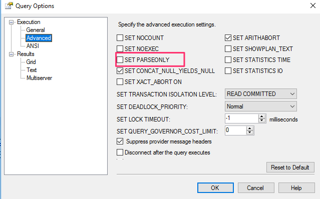
The Algebrizer parse and binds the SQL queries. It validates the syntax and uses the query information to build a relation query tree. Parsing only checks for valid SQL syntax without accessing the table names or columns or checking for their existence.

We can test the following in SMSS by setting the options to PARSE_ONLY

SELECT lname, fname FROM authors

The above will pass the syntax since that’s valid SQL statement.

The next stage is the binding, which validates the existence of the tables and their columns against the system catalogs and the permissions. The output is a algebrizer tree that is sent to the optimizer for optimization.

The tree contains logical operations that are closely related to the corresponding SQL statement. There is no documentation on this but there’s a DMV that have some information on the mappings of the logical operations :

SELECT * FROM sys.dm_xe_map_values 
WHERE name = 'query_optimizer_tree_id'

There are also several undocumented trace flags that can allow you to see these different logical trees. For example, you can use the following query with the undocumented trace flag 8605. But first enable trace flag 3604, as shown next:

DBCC TRACEON(3604)

and check in the message tab for the logical query tree :

SELECT * FROM Sales.SalesOrderDetail
WHERE SalesOrderID = 43659
OPTION (RECOMPILE, QUERYTRACEON 8605, QUERYTRACEON 3604)

The tree gets verbose quickly even for a small query. Unfortunately, there is no documented information to help understand these output trees and their operations.

Simplification

At this stage of the optimization process the query tree is simplified into a simpler form to enable quick optimization. Here are some of the things that happens during the simplification stage :

• Contradictions are detected and removed and SQL server will not even execute the query. The optimizer can detect that no row will be returned by using a certain set of predicate combination.
• Filters in the WHERE clause are pushed down the tree so that they are evaluated early and reduce the amount of data access and also enable using indexes to retrieve the data. This is called predicate pushdown.
• Subqueries are converted into joins if possible.
• Redudant inner and outer joins are removed, e.g in when a table is join with another table that have a foregin key relationship, the other table might not be needed to retrieve data in what is called a Foreign Key Join elimination.

Contradiction Detection

Let’s use a table with a check constraint and see how the optimizer does contradicition detection. There’s a check constraint on the HumanResources.Employee called CK_Employee_VacationHours. This constraint uses the following rule ([VacationHours]>=(-40) AND [VacationHours]<=(240)). The value needs to be between -40 and 240.

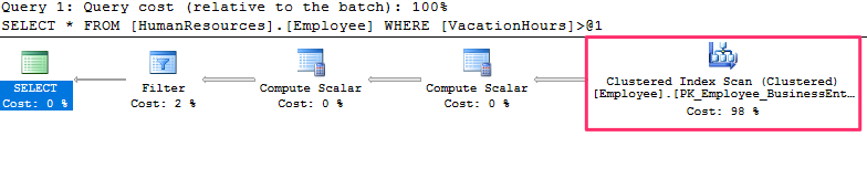
Let run the following query and look at the query plan :

SELECT * FROM HumanResources.Employee
WHERE VacationHours > 80

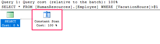
SQL Server will use a clustered index scan to retrieve the results, now lets change the value to 300 as follows :

SELECT * FROM HumanResources.Employee
WHERE VacationHours > 300

The query plan changes and SQL server now uses a constant scan and the table is not even accessed at all. Because there is no need to access the table at all, SQL Server saves resources such as I/O, locks, memory, and CPU, thus making the query execute faster.

Disable the constraint and run again and the index will now be scanned :

ALTER TABLE HumanResources.Employee NOCHECK CONSTRAINT CK_Employee_VacationHours

Enable the index back again :

ALTER TABLE HumanResources.Employee WITH CHECK CHECK CONSTRAINT CK_Employee_VacationHours

Another contradiction is when the predicate does contain the contradiction as follows :

SELECT * FROM HumanResources.Employee 
WHERE VacationHours > 10 AND VacationHours < 5

A trivial plan might also be used instead of a constant scan operator.

View the Simplified Tree

Using the undocumented query hint from before, we can examine the generated simplified query tree by running following query and looking at the messages tab :

SELECT * FROM HumanResources.Employee
WHERE VacationHours > 300
OPTION(RECOMPILE, QUERYTRACEON 8606,QUERYTRACEON 3604)

Here is the output truncated :

*** Input Tree: ***
        LogOp_Project QCOL: [AdventureWorks2012].[HumanResources].[Employee].BusinessEntityID QCOL: [AdventureWorks2012].[HumanResources].
            LogOp_Select
*** Simplified Tree: ***
LogOp_ConstTableGet (0) COL: IsBaseRow1000  QCOL: [AdventureWorks2012].[HumanResources].[Employee].BusinessEntityID QCOL:

Foreign Key Join Elimination

For the demonstration run the following query and observe the execution plan :

SELECT soh.CustomerID, c.AccountNumber
FROM Sales.SalesOrderHeader soh
JOIN Sales.Customer c
on soh.CustomerID = c.CustomerID

Here is the generated execution plan :

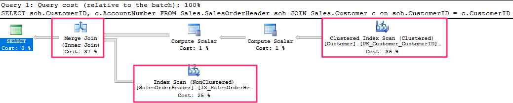
You will notice a merge join was used and both tables are read.

Now comment out the AccountNumber column and run the query again :

SELECT soh.CustomerID --, c.AccountNumber
FROM Sales.SalesOrderHeader soh
JOIN Sales.Customer c
on soh.CustomerID = c.CustomerID

and here is the generated execution plan :

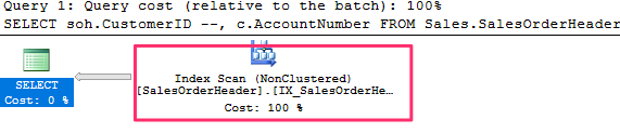
Notice that only Sales.SalesOrderHeader table is being read. The optimizer simplified the query using the foreign key constraint and in this case we do not need any rows from the Customers table so there is no need to access the table at all, and the foreign key guarantees the data returned is correct.

We can inspect the logical query tree using the trace flags :

SELECT soh.CustomerID --, c.AccountNumber
FROM Sales.SalesOrderHeader soh
JOIN Sales.Customer c
on soh.CustomerID = c.CustomerID
OPTION(RECOMPILE, QUERYTRACEON 8606,QUERYTRACEON 3604)

and the generated query tree truncated looks as follows :

*** Simplified Tree: ***
        LogOp_Join

            LogOp_Get TBL: Sales.SalesOrderHeader(alias TBL: soh) Sales.SalesOrderHeader

            LogOp_Get TBL: Sales.Customer(alias TBL: c) Sales.Customer

*******************
*** Join-collapsed Tree: ***
        LogOp_Get TBL: Sales.SalesOrderHeader(alias TBL: soh) Sales.SalesOrderHeader

Notice the simplified query tree still retrieves from both tables but the join collapsed tree only retrieves the data from one table.

Try disabling the constraint and run the query, you will notice the generated plan have to use the join as there is no other way to retrieve the data.

TRIVIAL PLAN

The optimizer chooses a trivial plan when there’s no other way to run the query. SQL Server uses it to avoid the expensive operation of query optimization for queries that does not involve any cost estimation, e.g the following query will use a trivial plan :

-- for example, testing with a very simple AdventureWorks2012 query, such as
SELECT * FROM Sales.SalesOrderDetail
WHERE SalesOrderID = 43659

The reason is being the there’s a unique index PK_SalesOrderDetail_SalesOrderID_SalesOrderDetailID that can only contain 0 or 1 row. We can use a trace flag 8757 to disable the use a trivial plan as follows :

-- let’s again add the undocumented trace flag 8757 to avoid a trivial plan
SELECT * FROM Sales.SalesOrderDetail
WHERE SalesOrderID = 43659
OPTION (RECOMPILE, QUERYTRACEON 8757)

and you notice from the properties in SSMS that we get a full optimization. Use the sys.dm_exec_query_optimizer_info and check the optimization information. You will notice instead of a trivial optimization, we have a hint and the optimization goes to search 1.

Now use a different column and you will get full optimization :

SELECT * FROM Sales.SalesOrderDetail
WHERE ProductID = 870

The reason is because they are several plans available and the query optimizer need to find the optimal plan to execute the query.

STATISTICS

The optimizer maintains statistics on columns and indexes that it uses during costing in the optimization process.

Query Operators

The operators or iterators are used by the execution engine to perform the operation of retrieving data based on the execution plan. The operators have different characteristics, some are memory consuming, and some have to build the input before they start executing. In this section we will look at the common operators using the execution engine.

Data Access Operators

These are the most common operators as they are used to retrieve data :

• Heap Table Scan
• Clustered Index Scan
• Clustered Index Seek
• Non-clustered Index Scan

• Non-Clustered Index Seek

• A scan reads an entire structure, which could be a heap, a clustered index, or a nonclustered index.

• A seek, on the other hand, does not scan an entire structure, but instead efficiently retrieves rows by navigating an index. Can only be performed on a clustered on nonclustered index.

Scans

Let’s start with the simplest example, by scanning a heap, which is performed by the Table Scan operator

-- the following query on the AdventureWorks2012 database will use a Table Scan
SELECT * FROM DatabaseLog

Similarly, the following query will show a Clustered Index Scan operator :

SELECT * FROM Person.Address

The scan operator does not guarantee returning sorted results. The storage engine uses efficient methods to return the data without sorting. Some features are only available in the Enterprise Edition. You can check the properties of the query plan to see if the results were return sorted by looking at the Ordered property.

Run the following and check the Ordered property :

-- if you want to know whether your data has been sorted, the Ordered property can show if the data 
SELECT * FROM Person.Address
ORDER BY AddressID

and you will notice that its now true.

Non-clustered index scan

The following query will produce a non-clustered index scan. The data will be returned without querying the base table :

SELECT AddressID, City, StateProvinceID
FROM Person.Address

Each non-clustered index contains a clustering key, so in this case we didn’t have to query the base table because the index also contains the clustering key.

Seeks

An Index Seek does not scan the entire index, but instead navigates the B-tree index structure to quickly find one or more records. These can be performed by both the Clustered Index Seek and the Index Seek operators.

The following query produces a clustered index seek :

 -- now let’s look at Index Seeks
SELECT AddressID, City, StateProvinceID FROM Person.Address
WHERE AddressID = 12037

and the following produces a non-clustered index seek :

-- the next query and Figure 4-6 both illustrate a nonclustered Index Seek operator
SELECT AddressID, StateProvinceID FROM Person.Address
WHERE StateProvinceID = 32

a clustered index seek can also return multiple rows, e,g in the following query :

-- the previous query just returned one row, but you can change it to a new parameter like in the following example:
SELECT AddressID, StateProvinceID FROM Person.Address
WHERE StateProvinceID = 9

The query have been auto-parameterized, so any query will use the same plan, we can try to drop the cached query plans but you will notice the same query plan will be used.

DBCC FREEPROCCACHE
GO
Use AdventureWorks2012
GO
-- the previous query just returned one row, but you can change it to a new parameter like in the following example:
SELECT AddressID, StateProvinceID FROM Person.Address
WHERE StateProvinceID = 9

The query is using a partial ordered scan. It first finds the initial row and continues scanning the index for all matching rows which are logically together in the same leaf pages on the index. In this case, the data was retrieved without ever touching the base table.

A more complicated example of partial ordered scans involves using a nonequality operator or a BETWEEN clause, like in the following example:

-- a more complicated example of partial ordered scans involves using a nonequality operator or a BETWEEN clause
SELECT AddressID, City, StateProvinceID FROM Person.Address
WHERE AddressID BETWEEN 10000 and 20000

A Clustered Index Seek operation will be used to find the first row that qualifies to the filter predicate and will continue scanning the index, row by row, until the last row that qualifies is found. More accurately, the scan will stop on the first row that does not qualify.

Bookmark Lookup

The bookmark operator is used when a nonclustered index is useful to find one or more rows but does not cover all the columns in the query. Because the nonclustered index contains the clustering key, the base table is accessed using the clustering key to retrieve the columns not covered by the index.

For example, in our previous query, an existing nonclustered index covers both AddressID and StateProvinceID columns. What if we also request the City and ModifiedDate columns on the same query? This is shown in the next query, which returns one record :

SELECT AddressID, City, StateProvinceID, ModifiedDate
FROM Person.Address
WHERE StateProvinceID = 32

The query optimizer is choosing the index IX_Address_StateProvinceID to find the records quickly. However, because the index does not cover the additional columns, it also needs to use the base table (in this case, the clustered index) to get that additional information. This operation is called a bookmark lookup.

Text and XML plans can show whether a Clustered Index Seek operator is performing a bookmark lookup by looking at the LOOKUP keyword and Lookup attributes :

SET SHOWPLAN_TEXT ON
GO
SELECT AddressID, City, StateProvinceID, ModifiedDate
FROM Person.Address
WHERE StateProvinceID = 32
GO
SET SHOWPLAN_TEXT OFF
GO

output :

StmtText
----------------------------------------------------------------------------------------------------------------------------------------
  |--Nested Loops(Inner Join, OUTER REFERENCES:([AdventureWorks2012].[Person].[Address].[AddressID]))
       ....
       |--Clustered Index Seek(OBJECT:.. SEEK:([Person].[Address].[AddressID]) LOOKUP ORDERED FORWARD)

(3 row(s) affected)

Now run the same query, but this time, request StateProvinceID equal to 20. Now this will produce an index scan :

SELECT AddressID, City, StateProvinceID, ModifiedDate
FROM Person.Address
WHERE StateProvinceID = 20

So the query optimizer is producing two different execution plans for the same query, with the only difference being the value of the StateProvinceID parameter. In this case, the query optimizer uses the value of the query’s StateProvinceID parameter to estimate the cardinality of the predicate as it tries to produce an efficient plan for that parameter.

The bookmark lookup performs random I/O so it is an expensive operation when more records need to be returned, so the optimizer instead chose to scan the index. The optimizer is cost based, so it used the statistics to find an optimal plan.

Aggregations

SQL Server have two physical operators for implementing aggregations :

• Stream Aggregate
• Hash Aggregate

Sorting and Hashing

Lets discuss sorting and hashing before continuing with the rest of the operators as this plays an important roles. The optimizer employs different methods to provide sorted data :

• Use an index
• use the Sort operator
• Use hashing algorithms

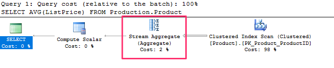
Stream Aggregate

The Stream Aggregate is used for scalar aggregates, aggregates that return only a single value, e.g the SUM, COUNT, AVG, ect.c functions.

SELECT AVG(ListPrice) FROM Production.Product

and produces the following plan :

Use the ext plan to reveal more information :

SET SHOWPLAN_TEXT ON
GO
SELECT AVG(ListPrice) FROM Production.Product
GO
SET SHOWPLAN_TEXT OFF
GO

• In order to implement the AVG aggregation function, the Stream Aggregate is computing both a COUNT and a SUM aggregate, the results of which will be stored in the computed expressions Expr1003 and Expr1004, respectively.
• The Compute Scalar verifies that there is no division by zero by using a CASE expression.

Group By Clause

When using a GROUP BY clause, the input needs to be sorted first, if not an operator is introduced to sort the results first :

-- now let’s see an example of a query using the GROUP BY clause
SELECT ProductLine, COUNT(*) FROM Production.Product
GROUP BY ProductLine

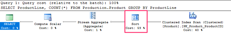
The first query did not use a sort operator because without a GROUP BY clause, the input is considered a single group.

Sort with an Index

The Stream Aggregate can also use an index to provide sorted results :

-- a Stream Aggregate can also use an index to have its input sorted, as in the following query
SELECT SalesOrderID, SUM(LineTotal)FROM Sales.SalesOrderDetail
GROUP BY SalesOrderID

output :

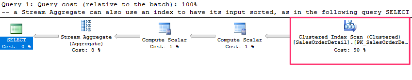
No Sort operator is needed in this plan because the Clustered Index Scan provides the data already sorted by SalesOrderID, which is part of the clustering key of the SalesOrderDetail table

Hash Aggregate

Its implemented with the Hash Match physical operator.

• Works on unsorted data for big tables
• Cardinality estimates should produce few groups
• Builds a hash table in memory

For example, the SalesOrderHeader table has no index on the TerritoryID column, so the following query will use a Hash Aggregate operator.

-- for example, the SalesOrderHeader table has no index on the TerritoryID column, 
-- so the following query will use a Hash Aggregate operator
SELECT TerritoryID, COUNT(*)
FROM Sales.SalesOrderHeader
GROUP BY TerritoryID

and produces the following output :

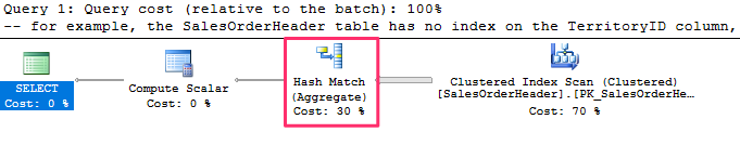
The algorithm for the Hash Aggregate operator is similar to the Stream Aggregate, with the exceptions that, in this case, the input data does not have to be sorted, a hash table is created in memory, and a hash value is calculated for each row processed.

When data is sorted the optimizer might choose a stream aggregate instead, try the following :

-- run the following statement to create an index
CREATE INDEX IX_TerritoryID ON Sales.SalesOrderHeader(TerritoryID)

and re-run the query. Notice the stream aggregate is now used, as the index is providing sorted input.

Drop the index when done :

-- to clean up, drop the index using the following DROP INDEX statement:
DROP INDEX Sales.SalesOrderHeader.IX_TerritoryID

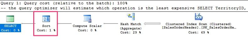
If the input is not sorted and order is explicitly requested in a query, the query optimizer may introduce a Sort operator and a Stream Aggregate, as shown previously, or it may decide to use a Hash Aggregate and then sort the results as in the following query :

-- the query optimizer will estimate which operation is the least expensive
SELECT TerritoryID, COUNT(*)
FROM Sales.SalesOrderHeader
GROUP BY TerritoryID
ORDER BY TerritoryID

and the plan produced :

Distinct Sort

A query using the DISTINCT keyword can be implemented by a :

• Stream Aggregate
• Hash Aggregate
• Distinct Sort operator

The Distinct Sort operator is used to both remove duplicates and sort its input. In fact, a query using DISTINCT can be rewritten as a GROUP BY query, and both can generate the same execution plan.

The following two queries return the same data and produce the same execution plan :

-- the following two queries return the same data and produce the same execution plan
SELECT DISTINCT(JobTitle)
FROM HumanResources.Employee
GO
SELECT JobTitle
FROM HumanResources.Employee
GROUP BY JobTitle

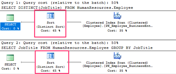
Note that the plan is using a Distinct Sort operator. This operator will sort the rows and eliminate duplicates.

If we create an index, the query optimizer may instead use a Stream Aggregate operator because the plan can take advantage of the fact that the data is already sorted. To test it, run this:

CREATE INDEX IX_JobTitle ON HumanResources.Employee(JobTitle)

Then run the previous two queries again. Both queries will now produce a plan showing a Stream Aggregate operator. Drop the index before continuing by using this statement:

DROP INDEX HumanResources.Employee.IX_JobTitle

Finally, for a bigger table without an index to provide order, a Hash Aggregate may be used, as in the two following examples:

-- finally, for a bigger table without an index to provide order, a Hash Aggregate may be used, as in the two following examples:
SELECT DISTINCT(TerritoryID)
FROM Sales.SalesOrderHeader
GO
SELECT TerritoryID
FROM Sales.SalesOrderHeader
GROUP BY TerritoryID

Join Operators

SQL Server uses three physical join operators to implement joins :

• Nested Loops Join
• Merge Join
• Hash Join

Nested Loops Join

The optimizer uses the Nested Join for workloads with a small resultset. Lets us the following query and see the query plan :

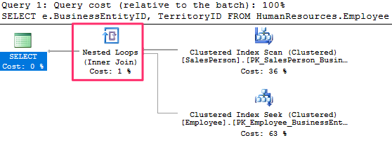
SELECT e.BusinessEntityID, TerritoryID
FROM HumanResources.Employee AS e
JOIN Sales.SalesPerson AS s ON e.BusinessEntityID = s.BusinessEntityID;

Notes of the Nested Loop

• Smaller results
• The operator used to access the outer input is executed only once
• The operator used to access the inner input is executed once for every record that qualifies on the outer input
• The outer table is shown on top in the graphical query plan

_

This query produces a plan similar to the one shown previously using the SalesPerson as the outer input and a Clustered Index Seek on the Employee table as the inner input. The filter on the SalesPerson table is asking for TerritoryID equal to 1, and only three records qualify this time. As a result, the Clustered Index Seek, which is the operator on the inner input, is executed only three times. You can verify this information by looking at the properties of each operator, as we did for the previous query.

SET STATISTICS PROFILE ON
GO
-- let’s change the query to add a filter by TerritoryID:
SELECT e.BusinessEntityID, HireDate
FROM HumanResources.Employee AS e
JOIN Sales.SalesPerson AS s ON e.BusinessEntityID = s.BusinessEntityID
WHERE TerritoryID = 1
GO
SET STATISTICS PROFILE OFF

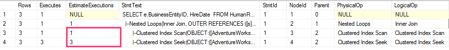
The query optimizer is more likely to choose a Nested Loops Join when the outer input is small and the inner input has an index on the join key. This join type can be especially effective when the inner input is potentially large, as only a few rows, indicated by the outer input, will be searched.

Merge Join

the Mere Join have the following characteristics :

• The optimizer chooses for medium workloads
• Requires sorted inputs
• Requires an equality operator
• Can use an index to provide sorted inputs
• Reads the inputs only once

Lets look at an example :

SELECT h.SalesOrderID, s.SalesOrderDetailID, OrderDate
FROM Sales.SalesOrderHeader h
JOIN Sales.SalesOrderDetail s ON h.SalesOrderID = s.SalesOrderID

and produces the following plan :

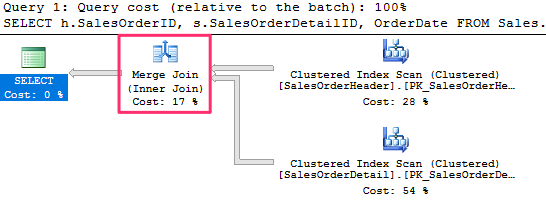
Taking benefit from the fact that both of its inputs are sorted on the join predicate, a Merge Join simultaneously reads a row from each input and compares them. If the rows match, they are returned. If the rows do not match, the smaller value can be discarded—because both inputs are sorted, the discarded row will not match any other row on the other input table.

If the inputs are not already sorted, the query optimizer is not likely to choose a Merge Join. However, it might decide to sort one or even both inputs if it deems the cost is cheaper than the alternatives. Let’s follow an exercise to see what happens if we force a Merge Join on, for example, a Nested Loops join plan.

-- if you run the following query, you will notice that it uses a Nested Loops Join
SELECT * FROM Sales.SalesOrderDetail s
JOIN Production.Product p ON s.ProductID = p.ProductID
WHERE SalesOrderID = 43659

and produces the following plan :

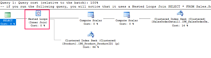
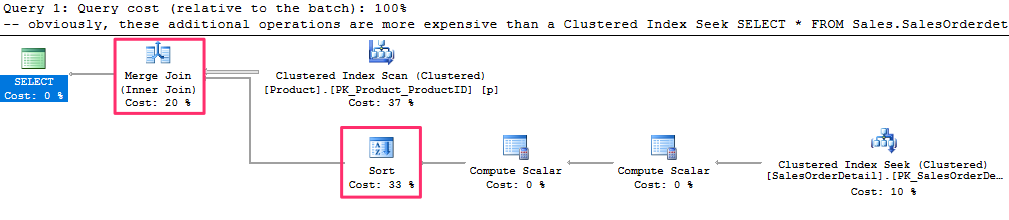
In this case, a good plan is created using efficient Clustered Index Seek operators. If we force a Merge Join using a hint, as in the following query, the query optimizer has to introduce sorted sources such as Clustered Index Scan and Sort operators, both of which can be seen on the plan

-- obviously, these additional operations are more expensive than a Clustered Index Seek
SELECT * FROM Sales.SalesOrderdetail s
JOIN Production.Product p ON s.ProductID = p.ProductID
WHERE SalesOrderID = 43659
OPTION (MERGE JOIN)

produces the following plan :

In summary, given the nature of the Merge Join, the query optimizer is more likely to choose this algorithm when faced with medium to large inputs, where there is an equality operator on the join predicate, and the inputs are sorted.

Hash Join

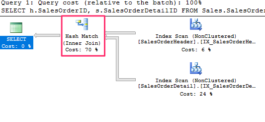
The query optimizer uses hash joins to process large, unsorted, non-indexed inputs efficiently. Lets run an example :

SELECT h.SalesOrderID, s.SalesOrderDetailID FROM Sales.SalesOrderHeader h
JOIN Sales.SalesOrderDetail s ON h.SalesOrderID = s.SalesOrderID

which produces the following plan :

Characteristics

• The Hash Join requires an equality operator on the join predicate,
• Unlike the Merge Join, it does not require its inputs to be sorted
• In addition, the operations in both inputs are executed only once
• Hash Join works by creating a hash table in memory
• The query optimizer will use cardinality estimation to detect the smaller of the two inputs, called the build input, and will use it to build a hash table in memory
• If there is not enough memory to host the hash table, SQL Server can use a workfile in tempdb, which can impact the performance of the query.
• A Hash Join is a blocking operation, but only during the time the build input is hashed
• After the build input is hashed, the second table, called the probe input, will be read and compared to the hash table

In summary, the query optimizer can choose a Hash Join for large inputs where there is an equality operator on the join predicate. Because both tables are scanned, the cost of a Hash Join is the sum of both inputs.

References

• https://msdn.microsoft.com/en-us/library/ms191158(v=sql.110).aspx
• https://docs.microsoft.com/en-us/sql/relational-databases/system-dynamic-management-views/sys-dm-exec-query-optimizer-info-transact-sql